Aerodynamics
Author: Richard Kenney
Probably the most important feature in designing a Greenpower car is to minimise the drag caused by the car moving through the air as it goes round the track, or aerodynamics. To some extent this can be done intuitively; for example it's obvious that a smaller car has to move less air aside than a larger car. Looking at the shapes of professionally designed cars and aircraft can also give some hints.
To get the best results intuition isn't enough and some tools are needed to help.
Optimisation Methods
In the past the only ways to work out the best shape for any body moving in a fluid (air, water etc) were to carry out manual calculations (complicated at best, practically impossible for a complex shape like a car) or to test models. To test a model you first have to actually build it (!) and then you need a way to accurately measure how it performs in the situation of interest. In our case this would mean building a wind tunnel and then measuring how much force is exerted on the model when air is flowing at a fixed speed. This is all a bit tricky - we have built the beginnings of a wind tunnel but we have yet to complete it, let alone work out how to calibrate the airflow and measure the force exerted on a model of a car when this is done.
Fortunately there is now another solution - simulation.
OpenFOAM
The simulator that we use is called OpenFOAM. It is a general purpose toolbox for solving CFD (computational fluid dynamics) problems which is very flexible and is used in many universities for simulating all sorts of problems where fluid movement is involved. For our use the advantages & disadvantages of OpenFOAM are:
Advantages
- It's free, as in open source - this means we afford to use it!
- Simulation results seem to make sense when compared with other tools, such as the system that Bentley use.
- The results can be viewed using Paraview which is a powerful graphical data analysis package.
Disadvantages
- It isn't the easiest program to use (there is no graphical front end, you have to use the command line).
- It is only available pre-compiled for Ubuntu Linux; we are running it under Linux but it may be possible to use the Linux subsystem in Windows 10.
- Because it is written for advanced users it takes some effort to understand how to set up the simulations correctly.
Using OpenFOAM
The basic steps to use OpenFOAM are:
- generate a surface model (STL file) of the car
- Setup a background grid mesh 'box' that is the volume to be simulated
- Create a mesh within the volume to represent the car
- Setup a simulation
- Run the simulation
- Analyse the simulation results
- Work out what should be changed to make things better
- Repeat until happy / fed up
Meshing
The left hand picture below shows the STL file exported from 3D CAD. The right hand picture shows the shape that was actually simulated. You can see that they are very similar but that there is some distortion as the meshing program (snappyHexMesh) generates a simulation grid matched as closely as possible to the shape of the car.
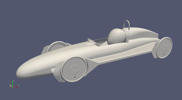 |
 |
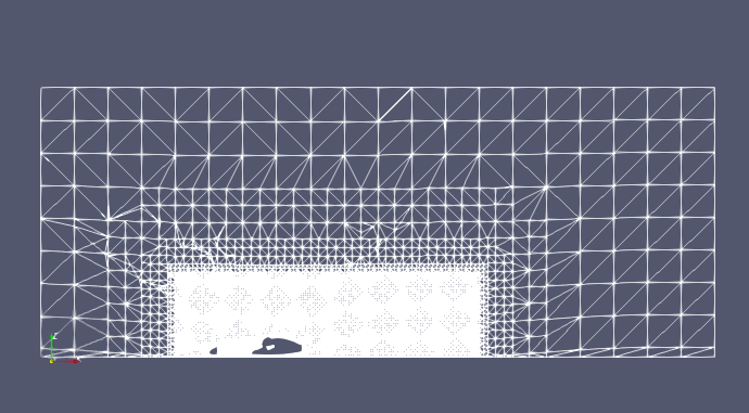
This picture shows a slice through the simulation grid at the centre of the car. You can see how the size of the grid cells gets bigger as the distance from the car increases.
Simulating
Once we have a model of the car ready to simulate we have to work out how to set up the simulator. This requires some understanding of how the simulation works.
Kinematic viscosity of air at 18ºC, \(\nu\)
\[\nu = 1.5 \times 10^{-5} \: \mathrm{m^2s^{-1}}\]
Speed of the car, \(|U_{ref}|\)
\[|U_{ref}| = 30.2 \: \mathrm{mph} = 30.2 \times \frac{1609.344}{3600} = 13.5 \: \mathrm{m\,s^{-1}}\]
The RMS turbulent air movement \(u'\) of the air through which the car is moving (this is estimated based on the rule of thumb that the turbulent movement of still air gives a turbulent intensity of less than \(1\%\) ).
\[u' = 0.1 \: \mathrm{m\,s^{-1}}\]
The length scale to be used in calculating the boundary layer turbulent flow around the car, \(L\), this is based on roughly the length of the car.
\[L = 2\:\mathrm{m}\]
Turbulence intensity of the air through which the car is moving
\[I \equiv \frac{u'}{|U_{ref}|} = \frac{0.1}{13.5} = 0.74\%\]
Now we can calculate the turbulence conditions \(k\) and \(\omega\) for the simulation model being used
\[k = \frac{3}{2} ( I\:|U_{ref}| )^2 = \frac{3}{2} \times ( 0.0074 \times 13.5 )^2 = 0.015\]
\[\omega = \frac{\sqrt{k}}{C_\mu L} = \frac{\sqrt{0.015}}{0.09 \times 2} = 0.68\]
Simulation File for Dylan
The link below is for an example simulation case with Dylan. By changing the STL file representing the car a comparable simulation can be run for other cars in order to understand whether the design is better or worse. To run the simulation, execute the Allrun script in the case folder. The Allclean script can be used to remove generated files if you want to re-run the simulation.
One point to bear in mind with the simulation is that it is currently set up to run using 4 cores in parallel. If the computer you will use has fewer cores than 4 then processes which run in parallel will exit with an error message complaining about the number of available slots - see the OpenFoam Manual Page for information about how to adjust this.
Sample simulation case with a model of Dylan
Comparing Simulations
How can we compare the results of the simulations? We need to define what is better or worse. In our case this is actually quite easy! All we care about is how hard the motor has to work to push the car through the air. This is defined by the drag on the car, and the simulation above includes data on this drag. All we have to do is plot the drag for each car to undestand how they compare. This has been done for our existing cars in the graph below.
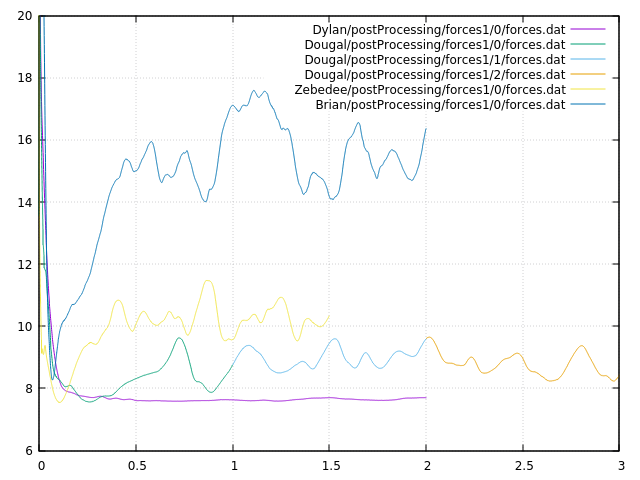
You can see that each car has been better than the one before and also that the airflow around Dylan is much more consistent (less turbulent) that previous cars.